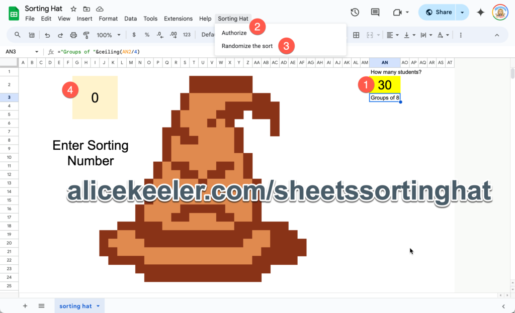

Just for fun!! Try this Google Sheets template to sort your students into the 4 houses of Hogwarts!
The template is available at alicekeeler.com/sheetssortinghat

Workshop: Gamified Warm-Ups
Go Slow workshop of 14 weeks of a gamified template each week along with directions for how to create that type of template.

Template: Sheets Sorting Hat (Harry Potter
Use this Google Sheets template to have a fun Hogwarts sorting activity with your students.

SimpleQuest: Gamified Google Form
SimpleQuest sets up a Google Form for students to do goal setting. MAKE IT A GAME! If you are interested in more join the Gamification

Desmos Polygraph – Engaging Activity
NOT MATH (and yes math) Desmos polygraph is an engaging vocabulary activity you can have your students play.

Create a Fun Bingo Activity
This fun Bingo Activity can be created for ANY subject. Get started with something fun.

Gamified Uno Sample
Try this Uno Warm-Up Sample and learn some tricks to speed up making your own!!

Spreadsheet Template
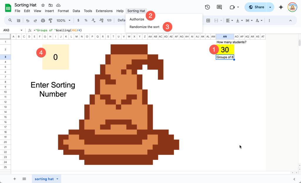
You know me, I love a spreadsheet! I used my Add-on for pixel art to insert a sheet where I could create the sorting hat. Typing single digit numbers I was able to fill the cell colors to recreate the hat. I did look up harry potter sorting hat pixel art on Google to find a pattern I could use.
Using the VIEW menu to remove the gridlines helps to create the illusion of the sorting hat.
How many Students?
The formula I used takes the number of students you enter into cell AN2 and divides it by 4… but of course, not all numbers divide evenly!!
The number of groups is =CEILING(AN2/4)
Ceiling always rounds up. If I have 11.25 groups… then I need 12 groups.
Evenly Balanced
When you enter in cell A2 that you have 41 students… you want these 41 students divided evenly amongst the 4 groups. There should be 11 students in each group although, only 10 will be assigned with one extra in a group.
I need a formula that creates 11 “Gryffindor’s” and 11 of the other 3 houses also.
I have the list of 4 houses in column A of a hidden sheet. Cell A2 has the value of “Gryffindor.”
=SPLIT(rept(A2,ceiling($C$2/4)),” “)
The formula REPT is repeat… so I want to repeat what is in cell A2 by the ceiling of the number of students divided by 4. However, this puts all the students into one cell. To split them out into individual cells I used the SPLIT function.
Now I have 11 of each group, but each in their own row. I use Transpose to turn this into columns.
To put this into a SINGLE column, the =FLATTEN(A14:D) formula does the trick. Notice my range ends in D and not D14. If I omit the row it will include the range for the entire column, below the initial starting row. Using Flatten takes each row (Gryffindor Hufflepuff Ravenclaw Slytherin) and turns into a column. So my column now alternates each of the 4 houses. Thus if I chose students 1, 2, 3, 4… I would have one student in each house. 5, 6, 7, 8… would have 2 students in each house. However, that is boring an predictable. The first student would always be Gryffindor as would the 5th student. You want more mystery!
So I added a random number next to each of the houses in the column. However, to sort by the random number I used an adjacent column to =SORT(G22:G). Now the list is randomly sorted and evenly balanced!!
=RAND() Updates on Edit
I love to use =RAND() or =RANDBETWEEN() however, the challenge is that each time you open the spreadsheet or edit anything, the rand randomizes again. That is no good as I want to randomize the list once and then go through the list to call on each student.
If I was using this only for myself I would simply highlight the randomized list, paste it into another column by using Control Shift V. The Shift key, when pasting, causes you to paste the VALUES instead of the formulas. Thus, I would have a list that is static after I randomized it.
However, I’m sharing this template and don’t want the user to have to do spreadsheet magic. Thus… Google Apps Script. So I coded a menu to allow you to copy the randomized list and paste the values. It’s what I said I would do manually, but you can do it much faster with the menu option!
I Hid My Messy Sheet
TBH I got sucked into this project. I was just thinking what formula would accomplish a sorting hat and it turned into a “if you give a mouse a cookie” situation. So then I went full in and made the pixel art sorting hat and the template. At first I was just messing around so I wasn’t trying to be well organized on my spreadsheet. If you look at my hidden sheet you will see it is a mess! Why is it organized like this? Well… it’s not organized. If I made this from scratch I would definitely do this better and more efficiently. But… TBH I don’t want to spend THAT much time on a sorting hat activity, hahaha.
Directions for Using the Template
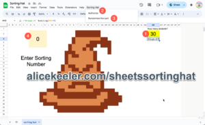
You do NOT need to know all the stuff I told you above to be able to use the template. I just thought some of you might be interested in how I made it. Basics are, make a copy of the spreadsheet. Put the number of students. Authorize and randomize the sort. Enter the sequential numbers for each student to reveal what house they are in.
Using the Template in Class
Before using with students, enter the number of students and run the code to sort the houses randomly.
In class, display the spreadsheet on the board so the students can see the sorting hat. If you can, find some Harry Potter sound effects on your phone to make this a little more jazzy.
In cell G2 enter the number 1. The first students sorting house will be revealed. Change the 1 to a 2 to reveal the 2nd students house. Be sure to celebrate and have fun with the sorting!!